Introduction to vauryou • vauryou

The vauryou package provides a collection of utilities, tools and standard components for VAÚ (Government Office of the Czech Republic). This vignette introduces the main functionality organized by topic.

Visual Identity and Colors

The package includes the official UV corporate colors and utilities for working with them.

Corporate Colors

# Individual UV colors
uv_cervena      # Corporate red
#> [1] "#802726"
uv_svetlemodra  # Light blue
#> [1] "#014D99"
uv_tmavemodra   # Dark blue
#> [1] "#150E43"
uv_stribrna     # Silver
#> [1] "#BEC0C2"
uv_seda         # Gray
#> [1] "#F2F2F2"
uv_logomodra    # Logo blue
#> [1] "#1E2047"

# Named vector of all UV colors
uv_cols
#>   logomodra        seda    stribrna svetlemodra  tmavemodra 
#>   "#1E2047"   "#F2F2F2"   "#BEC0C2"   "#014D99"   "#150E43"

Color Utilities

# Determine contrast colors for text readability
colors_to_test <- c("#802726", "#014D99", "#F2F2F2")
contrast(colors_to_test)
#> [1] "white" "white" "black"

# Custom contrast colors
contrast(colors_to_test, dark = "navy", light = "yellow")
#> [1] "yellow" "yellow" "navy"

Loading Colors from JSON

# Load color definitions from JSON file
# colors <- load_cols("colours.json")

Data Visualization with ggplot2

The package provides a comprehensive theming system and utilities for creating consistent visualizations.

VAU Theme

library(ggplot2)

# Basic plot setup
p <- ggplot(mpg) +
  geom_bar(aes(y = class)) +
  labs(title = "Vehicle classes", subtitle = "Count of cars by class")

# Apply VAU theme with y-axis gridlines (default)
p + theme_vau(family = "sans", title_family = "sans", gridlines = "y")
#> Warning: The `size` argument of `element_line()` is deprecated as of ggplot2 3.4.0.
#> ℹ Please use the `linewidth` argument instead.
#> ℹ The deprecated feature was likely used in the vauryou package.
#>   Please report the issue to the authors.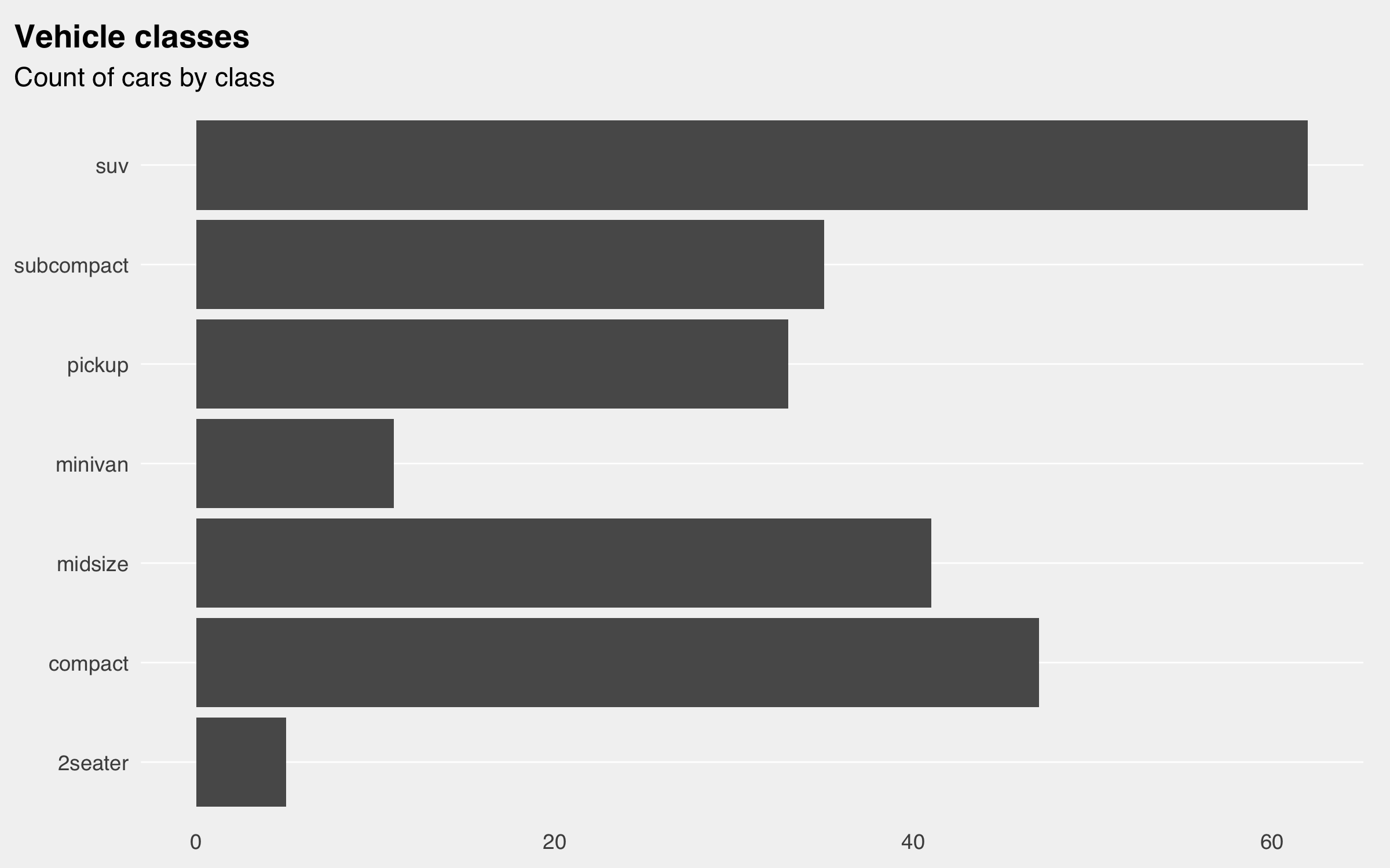

# Scatter plot styling
ggplot(mpg) +
  geom_point(aes(cty, hwy)) +
  theme_vau(gridlines = "scatter", family = "sans", title_family = "sans") +
  labs(title = "City vs Highway MPG", subtitle = "Fuel efficiency comparison")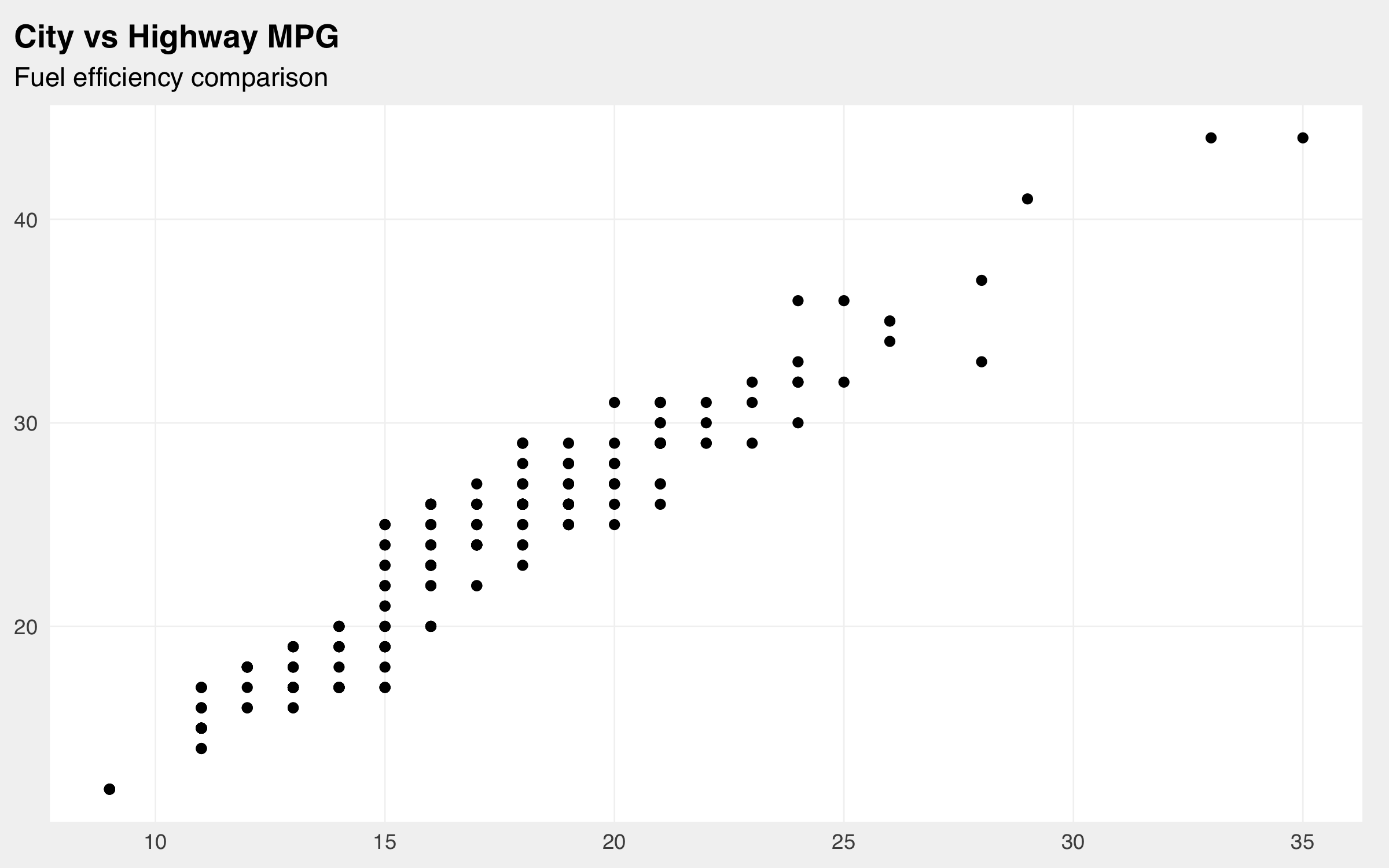

Axis Scaling and Formatting

The package provides Czech-localized scales with proper number formatting.

# Create sample data
sample_data <- data.frame(
  x = runif(50, 0, 100),
  y = runif(50, 0, 1)
)

ggplot(sample_data, aes(x, y)) +
  geom_point() +
  theme_vau(gridlines = "scatter", family = "sans", title_family = "sans") +
  scale_x_number_cz() +
  scale_y_percent_cz() +
  labs(title = "Czech formatting example", 
       subtitle = "Numbers with space separator, percents with comma")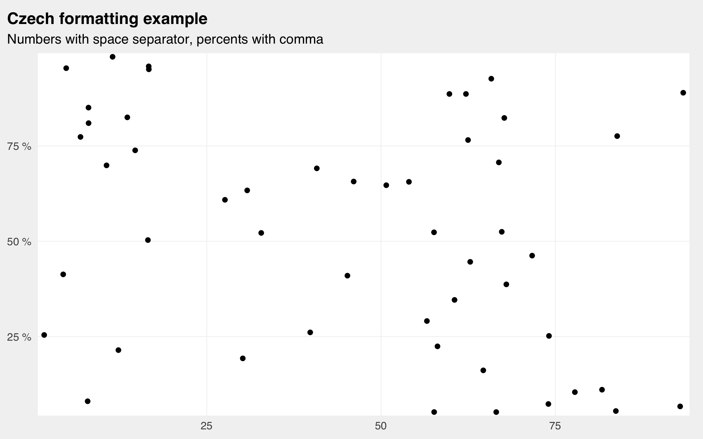

Custom Formatting Functions

# Format numbers with Czech conventions
numbers <- c(1234.56, 5678.90, 9876.54)
label_number_cz()(numbers)
#> [1] "1 235" "5 679" "9 877"

# Format percentages with Czech conventions  
percentages <- c(0.123, 0.456, 0.789)
label_percent_cz()(percentages)
#> [1] "12 %" "46 %" "79 %"

Visual Customization

# Set consistent defaults for geometric objects
set_geom_defaults(color = uv_logomodra)

# Set font defaults for text elements
set_vau_ggplot_fonts(family = "sans")

Axis Utilities

ggplot(mpg) +
  geom_bar(aes(y = class)) +
  theme_vau(family = "sans", title_family = "sans", gridlines = "x") +
  scale_x_continuous(expand = flush_axis()) +
  labs(title = "Classes with flush axis", subtitle = "No padding on x-axis")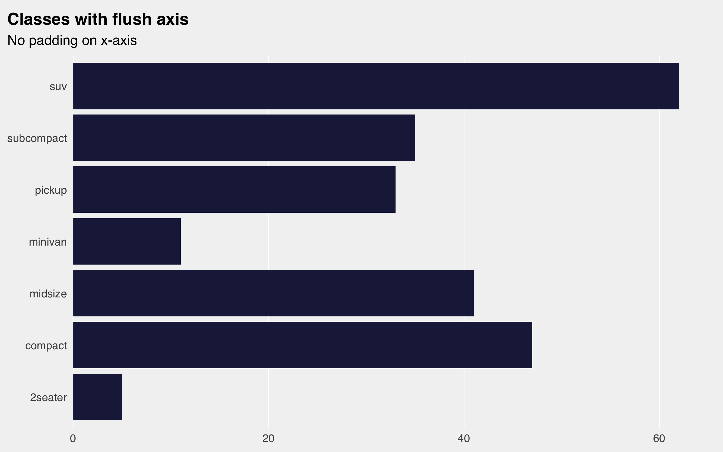

Saving Plots

# Save plots with standard VAU settings
p <- ggplot(mpg, aes(cty, hwy)) +
  geom_point() +
  theme_vau(family = "sans", title_family = "sans")

# Save to configured charts directory
save_png("fuel_efficiency", plot = p, width = 18, height = 9)

File Management and Paths

The package provides utilities for managing file paths and configurations.

Configuration-based Paths

Note these only work with a config.yml file in the directory.

# Get path based on config.yml settings
pth("charts", "my_plot.png")

# Path with subdirectory that will be created if needed
pth("data", "processed", "final_results.csv")

Package Files

# Get path to file included in the package
config_template <- vauryou_file("config.yml")

# Copy package files to project
copy_vauryou_file("config.yml", to = ".")
copy_config_template(to = ".")

Data Export and Documentation

Excel Workbook Creation

The package provides sophisticated Excel export capabilities with documentation support.

# Sample data
monthly_data <- data.frame(
  month = month.name[1:6],
  value = runif(6, 100, 1000),
  category = rep(c("A", "B"), 3)
)

annual_data <- data.frame(
  year = 2020:2023,
  total = runif(4, 5000, 10000)
)

# Documentation tables
guide <- data.frame(
  variable = c("value", "category", "total"),
  description = c("Monthly value in CZK", "Category classification", "Annual total"),
  type = c("numeric", "factor", "numeric")
)

codebook <- data.frame(
  code = c("A", "B"),
  meaning = c("Primary category", "Secondary category")
)

# Create comprehensive Excel workbook
write_nice_xlsx(
  output_path = "report.xlsx",
  data = list(
    "Monthly Data" = monthly_data,
    "Annual Summary" = annual_data
  ),
  documentation = list(
    "Variable Guide" = guide,
    "Category Codes" = codebook
  ),
  as_tables = TRUE,
  auto_width = TRUE
)

Configuration Management

The package integrates with the config package for environment-specific settings.

Example config.yml structure

default:
  base_dir: "."
  charts_dir: "charts"
  data_dir: "data"
  
production:
  base_dir: "/path/to/production"
  charts_dir: "outputs/charts"

Using Configuration

# Paths are automatically resolved using config.yml
chart_path <- pth("charts_dir", "my_chart.png")  # Uses charts_dir from config
data_path <- pth("data_dir", "processed.csv")    # Uses data_dir from config

# Manual subdirectory (creates charts/ under base_dir)
manual_path <- pth("charts", "manual_chart.png")

Complete Workflow Example

Here’s a complete example combining multiple package features:

# Set up plotting defaults
set_geom_defaults(color = uv_logomodra)
set_vau_ggplot_fonts(family = "sans")

# Create and style a plot
final_plot <- ggplot(mpg, aes(x = cty, y = hwy, color = class)) +
  geom_point(size = 2) +
  theme_vau(gridlines = "scatter", family = "sans", title_family = "sans") +
  scale_x_number_cz() +
  scale_y_number_cz() +
  scale_color_manual(values = rep(uv_cols, length.out = length(unique(mpg$class)))) +
  labs(
    title = "Fuel Efficiency Analysis",
    subtitle = "City vs Highway MPG by vehicle class",
    x = "City MPG",
    y = "Highway MPG",
    color = "Vehicle Class"
  )

# Save the plot
save_png("fuel_analysis", plot = final_plot, width = 20, height = 12)

# Prepare data for export
summary_data <- mpg %>%
  group_by(class) %>%
  summarise(
    count = n(),
    avg_cty = mean(cty),
    avg_hwy = mean(hwy),
    .groups = "drop"
  )

# Create documentation
data_guide <- data.frame(
  variable = c("class", "count", "avg_cty", "avg_hwy"),
  description = c("Vehicle class", "Number of vehicles", "Average city MPG", "Average highway MPG"),
  type = c("character", "integer", "numeric", "numeric")
)

# Export to Excel with documentation
write_nice_xlsx(
  output_path = pth("data", "fuel_analysis.xlsx"),
  data = list("Summary" = summary_data),
  documentation = list("Data Guide" = data_guide),
  as_tables = TRUE,
  auto_width = TRUE
)

Summary

The vauryou package provides:

Visual Identity: Official UV colors and contrast utilities
Visualization: Comprehensive ggplot2 theming with Czech localization
Data Export: Sophisticated Excel workbook creation with documentation
File Management: Configuration-based path handling and package file utilities
Workflow Integration: Seamless integration between visualization, export, and documentation

This creates a consistent and professional toolkit for data analysis and reporting within the VAÚ environment.